
Unconventional insight with InSAR.
In this second blog post on InSAR, I will look at if InSAR data could be used to map the surface deformation associated with unconventional stimulations. If you could, it would not a magic bullet, but could provide a different look at the response of the subsurface to the completion operation.
We know from data acquired using tiltmeters (a device placed on the ground surface, or in a wellbore, which measures tilt) that the process of creating fractures in the earth by stimulating a pad of multiple lateral wellbores, by pumping thousands of gallons of water and tons of sand into it, results in surface deformation. The question I want to discuss is whether this anomaly when measured with InSAR (spatially and temporally), can be related to the subsurface stimulated volume of rock and ultimately hydrocarbon production from that pad, lateral, and even perhaps stage.
We have known for some time that the energy we put into the ground during the stimulation is far greater than the energy of microseismic events we measure (by many orders of magnitude), this so called “seismic injection efficiency” might indicate the amount of surface deformation we might expect, I will show an example of this using public data from the MSEEL project later.
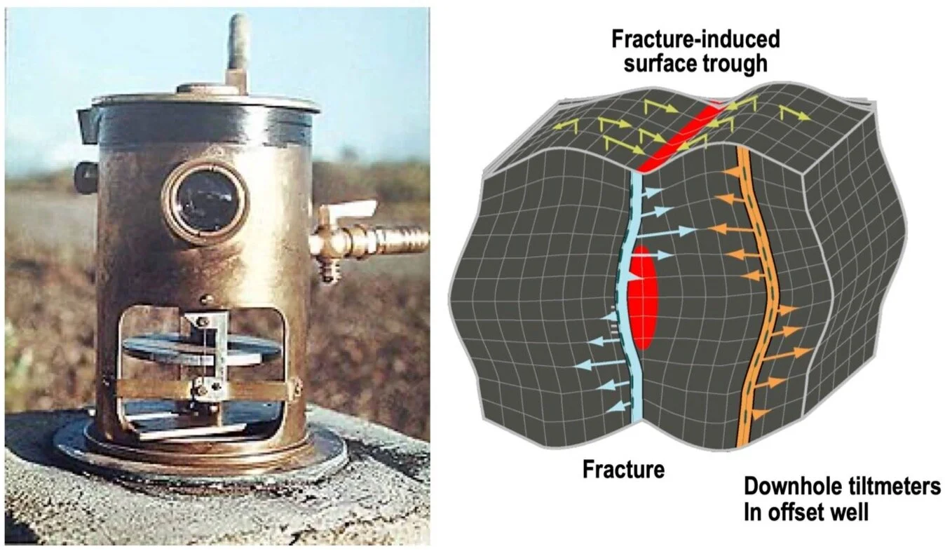
Surface Tiltmeter (left) and schematic of surface deformation induced by subsurface fracture network (right).
This is not an original idea. Rodriguez-Herrera et al (2017) used InSAR data to generate a 3D geomechanical model of a carbonate reservoir in Kuwait which was used to relate surface subsidence to pore pressure changes in the reservoir. However, from what I know this is not something that has been tested in the unconventional domain.
As a reminder, in case you didn’t read last weeks post, InSAR is a satellite technology used for measuring surface deformation, how much the ground surface rises or falls due to sub surface volume changes caused by fluid (or gas) injection or extraction. With ongoing improvements in temporal and spatial resolution, changes in the order of a millimeter/year can be measured. No land-based personnel or equipment are required, and no bespoke data acquisition is required. Historical data is available which could be useful for a proof-of-concept study such as what will be proposed here.
Ok so let’s put on our unconventional completions/exploitation engineers hats and talk about some key factors in unconventional resource development; well spacing, lateral length and stage spacing. Optimizing these elements (among others) is crucial for optimal production and ultimately, efficient field development. One of the commonly used measures to assess these elements is ‘stimulated rock volume’ or ‘drained rock volume’, or one of many other similar terms used to express the volume of rock which influences hydrocarbon production, either at the individual stage level, lateral level or pad level. Obviously, I choose my words carefully, the point is that whatever you call it, understanding how the time and money spent at the surface to stimulate a well related to ultimate production is important.
There are currently lots of methods used to understand this stimulated rock volume; radioactive tracers, image logs, core, tiltmeters, cuttings, and of course DTS/DAS VSP and microseismic, to name a few. Each measure different things, each contributing to the overall assessment. Morales et al (2019) describe an extensive, data rich project from the Eagle Ford utilizing many different sources of data to describe and optimize field development.
I would like to add another method to that list, InSAR.
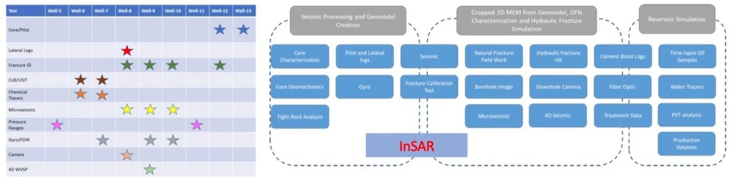
Data acquisition strategy for pad (left) and subsequent data integration work flow (right) modified from Morales et al (2019).
As an example of what might be possible, let’s consider the publicly available microseismic data from the Marcellus Shale Energy& Environmental Lab (MSEEL). The picture below shows all the microseismic events recorded, their color corresponds to the lateral, which was being stimulated when they were recorded, and their size is related to the moment magnitude of the event and hence the energy imparted to the formation. The microseismic data was acquired over a period of six days. The gross spatial dimensions of the microseismic events are shown. Does this area represent the stimulated area contributing to production? Likely not but it does offer unique insight into the fracture network created by the stimulation.

Map view of all microseismic events recorded during the stimulation of the MSEEL 5H well. Events are colored by the stage being stimulated when they were recorded and sized relative to their magnitude. Gross estimated dimensions of the microseismic event cloud is shown.
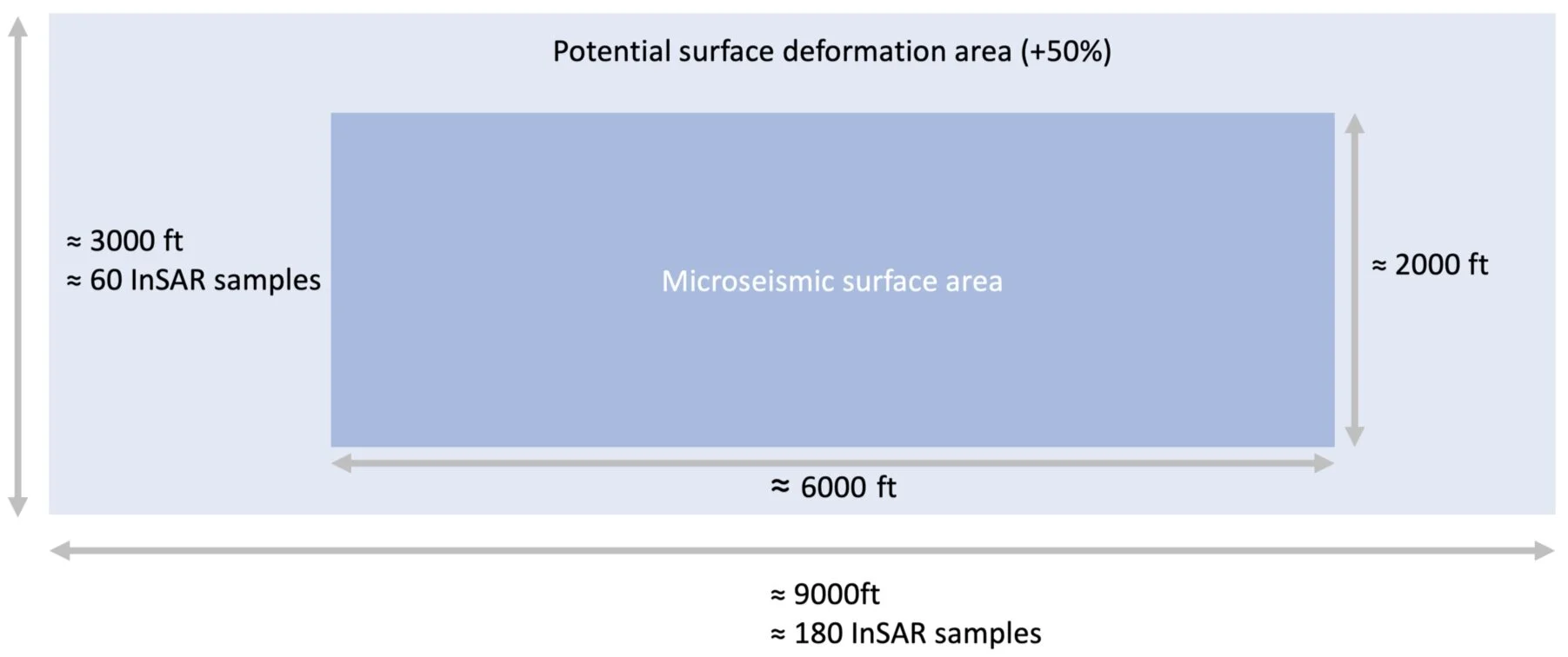
InSAR camping considerations based on microseismic event cloud dimensions.
Potential InSAR spatial samples at 50 ft sampling:
180 x 60 samples
Potential InSAR temporal samples:
6 days / 12 hours = 12 samples
Is it likely that this scale of subsurface alteration would result in a surface deformation signature that could be resolved with InSAR? Let’s assume that the deformation at the surface is 50% than at the reservoir level and that we have spatial InSAR resolution of about 50 ft and temporal resolution of about 12 hours you can see from the cartoon below that we should be able to acquire enough samples over the area influenced by the stimulation.
The question would be is the deformation large enough to be measured. If it was, we would be able to map the surface elevation changes with time as the subsurface fracture network developed throughout the stimulation.
Maxwell et al (2008) first discuss the idea of “seismic injection efficiency” as the ratio of the (micro)seismic energy to the hydraulic injection energy in relation to the concept of mass balance. They argue that the work done at the surface during stimulation can be estimated as the product of the injection pressure and the volume of injected fluid. To comply with the principle of energy conservation, this energy must be accounted for in the subsurface. Several processes are identified.
Heat
Friction
Fluid leak-off
Fracture creature and associated microseismicity
Interaction with existing fractures and potential seismicity
Surface dilation
They went on to show that the microseismic energy is a very small part of the total hydraulic energy with ratios between 1 x 10⁻⁹ and 1 x 10⁻⁵.
Seismic injection efficiency computed using surface (solid) and bottomhole (dashed) pumped energies (Maxwell et al, 2008).
Perhaps then including surface dilation measurements using InSAR data would provide a more complete picture of the impact of the hydraulic energy subsurface (ironically measured not even at the surface but from far above it from space).
The MSEEL data set, or other similar publicly available data set from an infield test lab (such as HFTS or HFTS-2) would provide excellent opportunities to test the idea. Unfortunately, I do not have access to the InSAR data but can make a start by looking at the seismic injection efficiency.
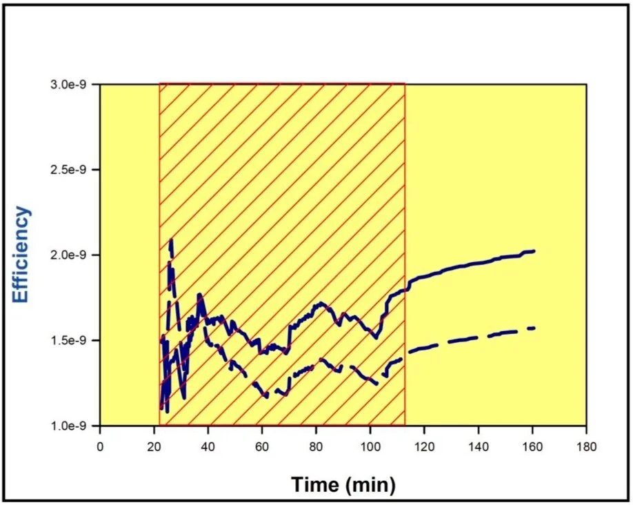
Using MSEEL pumping data from stage 23 of the 5H well I computed the seismic injection efficiency throughout the stage and compared the average seismic and hydraulic energies with those shown by Maxwell & Rutledge (2013) which include data from Canada and the UK. Interestingly, the MSEEL data for this stage shows a low seismic efficiency. Of course, doing this for all stages on all wells would give a more complete picture but for now I just wanted to demonstrate one example.
The pumping data from the stage is shown below along with a histogram showing when microseismic events were recorded, the initiation of microseismicity is quite typical with a large number of events early in the stage corresponding to fracture initiation.
The hydraulic injection energy of the stage is computed as the cumulative product of the slurry rate and treatment rate and the seismic energy as the cumulative sum of the seismic energy of individual microseismic events. Their ratio, the “seismic injection efficiency” is shown below, the blue shading corresponds to equivalent time periods. I also posted the stage average values on the examples provided by Maxwell and Rutledge (2013). It is interesting that this single stage plots amongst the more inefficient examples, perhaps reflecting a higher proportion of aseismic deformation. Analyzing the remaining data from this project would be interesting.
This is where one on the InSAR data processing companies need to step in and take a look at the data over the area for the given time period. Is deformation detectible, if so what magnitude and how does it evolve over the course of the stimulation. Let me know if you need the spatial coordinate and time range!
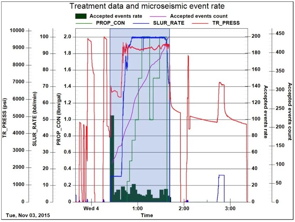
MSEEL 5H Stage 23 treatment data and microseismic event rate. Highlighted area corresponds to time duration of stage.
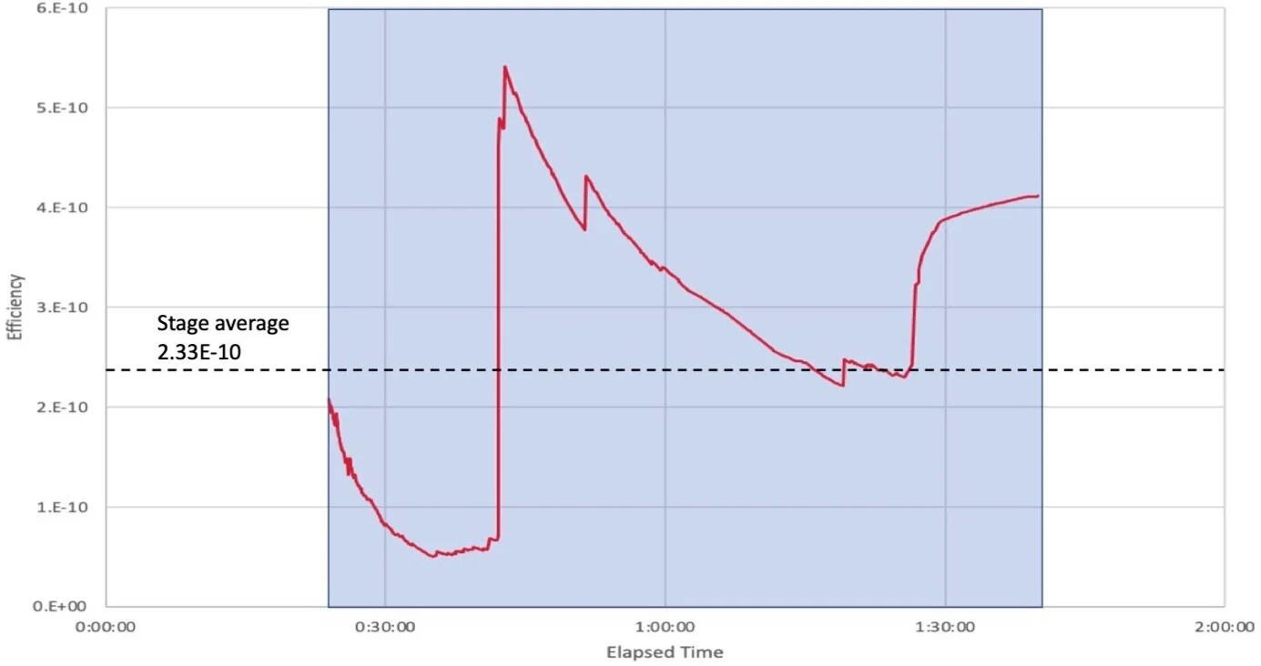
MSEEL 5H Stage 23 variation in seismic injection efficiency.
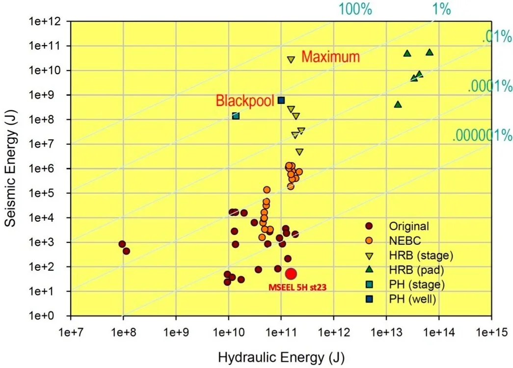
Crossplot of seismic versus hydraulic energy for various cases. MSEEL 5H stage 23 overlain (after Maxwell & Rutledge, 2013).
So, what would be the point of this? Even if you could use InSAR data to map the surface deformation associated with unconventional stimulations, how does it help? What would you do with it? Well, it’s not a magic bullet, InSAR would provide a different look at the response of the subsurface to the completion operation. Correlating surface deformation data, initially with microseismic data for calibration and then production data would be a first step. Beyond that perhaps there is a correlation between surface deformation and production. The real beauty of this data is that it already exists for completed pads and continues to be acquired with increasing resolution.
In an ideal world I am looking forward to reading about correlating InSAR with downhole data from the MSEEL or HFST or HFTS-2 datasets in TLE or FB or The Recorder ……
References
Jordan Ciezobka, et al. Hydraulic Fracturing Test Site (HFTS) – Project Overview and Summary of Results. URTEC, Houston, Texas, 23-25 July 2018.
E.A. Ejofodomi, et al. Using a Calibrated 3D Fracturing Simulator to Optimize Completions of Future Wells in the Eagle Ford Shale. URTeC: 2172668. URTEC, San Antonio, Texas, USA, 20-22 July 2015.
Adrian Rodriguez-Herrera et al. Inversion of satellite surface-deformation measurements over the Umm Gudair field, SEG Technical Program Expanded Abstracts: 3791-3795. 2017
Shawn Maxwell, et al. Microseismic deformation rate monitoring. SPE-116596. SPE Annual Technical Conference and Exhibition, Denver, 2008.
Shawn Maxwell, James Rutledge. Deformation investigations of induced seismicity during hydraulic fracturing. SEG Annual Meeting, Houston, 2013.
Robert Meek, et al. Time-Lapse imaging of a hydraulic stimulation using 4D Vertical Seismic profiles and fiber optics in the Midland Basin. URTEC, Austin, Texas, 24-26 July 2017.
Adrian Morales, et al. Case Study: Optimizing Eagle Ford Field Development Through a Fully Integrated Workflow. SPE-195951-MS, SPE Annual Technical Conference and Exhibition, Calgary, Alberta, Canada, 30 Sep - 2 October 2019.