Monitoring CO2 containment, part 2

Surface & Near Surface Monitoring

In this post I will continue with an overview of the elements of monitoring programs put in place to ensure that geologically sequestered carbon dioxide stays contained and does not leak to the surface. 

But first, I was distracted by an opinion piece from the folks at Wood Mackenzie recently which was shared on LinkedIn. Two things struck me, firstly the estimated size of the CCUS market globally. They estimate that the CCUS development pipeline, currently has 130 million tonnes per annum (Mtpa) of capture capacity. This will need to increase 184 fold to achieve the 1.5 °C pathway called for in the Paris Agreement on climate change. Now, we can discuss the ‘details’ behind that estimate but the fact remains, IMHO, that CCUS will grow significantly in the coming years. To put these numbers in some kind of perspective, the ongoing Quest project (Shell, Canada) and the now completed Weyburn project (Cenovus, Canada), between them, sequestered 5 Mtpa. The other point of interest in the article was the recognition that for this increase to be possible it will require the introduction of large-scale CCS hubs. Food for thought indeed.

So, in other words there is likely to be lots of demand for monitoring associated with these projects. As I mentioned in the first part of this discussion a few weeks ago, a monitoring program is required to satisfy the terms of the tax credit (45Q) associated with the geological storage of CO2. These programs can be divided into three main zones of investigation.

• Atmospheric

• Surface / near surface

• Subsurface

All CCUS MVA programs should have elements of each. For example, part of my research for this blog led me to a paper by Li et al (2014) from which I have taken their baseline MVA program and overlain these zones.

Suggestion of baseline monitoring framework for China's CCUS project with monitoring zone categories overlain. Adapted from Li et al (2014)

This post will discuss the methods and techniques employed to measure changes to the surface and near surface.

In some ways, the methods described in the previous post for monitoring leaked CO2 in the air, immediately above the ground, beneath which the CO2 has been stored, smacks of “shutting the door after the horse has bolted”. The fact you are measuring it at all, implies it has already escaped. But of course, as discussed, these would not be the only monitoring methods used.

Identifying elevated CO2 levels at, or near, the surface, provides a more manageable risk framework and allows more time for mitigation.

There are two broad categories of monitoring which fall into this section.

• Near surface geochemical monitoring of groundwater and soils

• Surface elevation changes 

Near surface geochemical monitoring of groundwater and soils

One of the major challenges with monitoring in this shallow, near surface zone is ensuring that whichever technique is used, it can differentiate between naturally occurring, and injected, CO2. Case in point, Kerr Farm, SK, Canada which lies to south east of the Weyburn CO2 injection area. To cut a (very) long story short, years of allegations of CO2 contamination, claims and counter claims, were ultimately unsatisfactorily resolved. However, two important lessons were learnt; the need for pre injection background monitoring for at least a year to capture seasonal variations in soil CO2 and the need for a published claim response protocol.

Moving on, there are several different geochemical techniques to estimate changes in CO2 levels in the soil, I will describe what I think might be the most useful method and mention a few others. 

Between 2008 and 2013, Total operated the Lacq-Rousse CO2 capture and storage demonstration project. Produced CO2 from the Lacq plant was injected into the fractured dolomite of the depleted Rousse field at a depth of approximately 4200m. A total of 51,000 tons of CO2 was injected. A thorough MMV, post injection monitoring program (required by regulation) was conducted until March 2016 encompassing (somewhat limited) atmospheric, surface and subsurface monitoring.

In an extremely interesting and comprehensive review, Gal et al (2019), describe the geochemical surface monitoring including the soil-gas concentrations and soil-gas flux monitoring part of that MMV program. The map below shows the layout of surface sample points, 20 measurements were taken at most locations between 2008 and 2015 covering the pre injection, injection, and post injection periods.  

Locations of the 36 monitoring stations (35 different locations) plotted onto a geological map. The hexagon shape links the six geophysical observation boreholes for passive seismic monitoring down to 2 km‐depth. Point 16‐A is close to the location of the injection well (RSE‐1).  (Gal et al, 2019)

Soil-gas concentrations were derived from samples collected at a depth of 1m and analyzed using an Infra-Red Gas Analyzer. Soil-gas flux was measured using a small, sealed chamber on the soil surface which measured gas movement over a period of a few minutes of circulation. The test was performed separately for CO2 and CH4.

INERIS flux chamber diagram (Pokryszka et al, 2000)

The interpretation of the dataset is, of course, complex. Environmental variables such as temperature, pressure and rainfall, and their interaction with the soil, varies naturally over time. The environmental data monitored at each station is shown below where the seasonal variations are clear.

Air temperature, soil water content and atmospheric pressure measured during each field session at each monitoring location. Data are shown as box plots presenting median value, quartiles and outliers (Gal et al, 2019).

Results of the 8 years of monitoring CO2 concentrations and CO2 flux are shown below, and to paraphrase the conclusions, the variations in CO2 concentrations and CO2 flux were due to seasonal and environmental changes, and not (by extension), leakage of injected CO2 from below.

Soil CO2 concentration, soil-gas flux at the soil/atmosphere interface (Gal et al, 2019)

A different approach to near surface geochemical monitoring of groundwater and soils is taken by Li et al (2014). They describe a shallow well monitoring system with U-tube sampling technology to measure gas and liquid composition at the Shengli oilfield CCUS demonstration project in China. This system is based on an earlier design implemented at the Frio brine aquifer in Liberty County, Texas through work funded by the DoE (Freifeld et al, 2005). At each test site a 10m wellbore is drilled and equipped with a series of isolation plugs and sampling chambers, each of which is part of its own U-tube collection system with a surface sampling bottle and nitrogen supply at both ends. At regular intervals the nitrogen forces the gas and liquid from the sampling chamber into the sampling bottle. This was, independent samples are collected from three different depths as shown. The challenge with this approach is that I expect it is very expensive, many test sites would be required, and drilling and equipment costs would probably be prohibitive.

Depiction of CO2 monitoring system in a shallow well (left) and schematic diagram of the U-tube sampler (right) (Li et al, 2014)

A novel, alternative method to identify elevated levels of escaped CO2 in the near surface is described by Kim et al (2019) who investigates the effect of CO2 on plant growth. In laboratory experiments they compare the effect of elevated CO2 conditions on the growth of corn compared with natural conditions. As you can see below the corn exposed to CO2 is stunted and generally looks quite unwell. The challenge I see with this approach is on the control side; not all corn will grow the same way even if all other variables are identical.

Design of growth box (a) and experimental arrangement (b), top. Morphology of corn leaves in the ‘CON’ (control) and CO2  (CO2  gas injection) treatments, bottom (Kim et al 2019).

Never wanting to miss a chance to show a fiber-optic (FO) example, Ahmed et al (2019), present an experimental study of an intriguing FO encapsulated sensor for CO2 monitoring. I am bringing this up here because the test results they show are from a shallow buried cable, however, the ambition appears to be that this cable can be deployed onshore and offshore downhole and on surface. Also, because I haven’t mentioned fiber for the last three blog posts!

The small hollow-core photonic sensor allows the gas to enter for analysis (below), the sensor is calibrated in the lab and is shown to be stable and repeatable for a variety of CO2 concentrations. The calibration provides the relationship between wavelength and CO2 concentration. Near surface deployment is tested by burying the sensor to a depth of 20cm in soil and exposing it to various concentrations of CO2. The lab results are impressive, and I am looking forward to reading about field deployment results.

Schematic of the Mach–Zehnder interferometer (MZI) constructed using a small stub of hollow-core photonic crystal fiber (HC-PCF), top, working principle based on geometric light propagation in the fiber assembly, middle. Schematic of packaging (a), and sensor packaging (b), bottom (Ahmed et al, 2019).

(a) Laboratory setup for CO2 concentration measurement in soil, and (b) measurement of CO2 concentrations in soil at atmospheric pressure and room temperature (Ahmed et al, 2019)

You could imagine, assuming conducive sensor economics, a grid of shallow (trenched) cable over the zone of injection with the ability to sample on demand. Oversimplification? Probably but I have no doubt it is being looked at by the main players in this domain.

 This brings us to, currently, my second favorite subject, InSAR.

Monitoring surface elevation changes with InSAR

The second element in this part of an MVA program is the potential use on InSAR to measure changes in surface elevation as a result of CO2 injection. As regular readers may know, I have become quite the fan of InSAR lately. The combination of a remote, contactless technology, with ever increasing resolution and continuous acquisition is compelling.

The poster child of using InSAR as part of a CCUS MVA program is the InSalah CCUS project in central Algeria which removed CO2 from several gas fields at a central gas processing facility and then compressed, transported and stored the liquid underground in the 1.9 km deep Carboniferous sandstone unit at the Krechba field (Rucci et al, 2018). Increased reservoir pressure caused by the CO2 injection ultimately resulted in surface deformation which was measured using InSAR. In a flat homogenous world this deformation would appear spherical and proportional in size to the injected volume. Of course, it’s not. The reservoir of the Krechba field is fractured and the increased reservoir pressure led to tensile failure and potentially, cap rock integrity issues. In this case the InSAR signature looks somewhat different. The displacement map below shows a two-lobe pattern over one of the lateral injector wells and is interpreted as an example of potential fault activation.

(Left image) Average displacement rate map [mm/yr] provided by the analysis of SAR data. The black line represents the location of the fault plane inferred by a geomechanical analysis. (Right image) Amount of tensile opening of the fault plane.

In another example from the Powder River basin, the Bell Creek project is demonstrating that commercial EOR operations can safely and cost-effectively store regionally significant amounts of CO2. Bell Creek Field owner, Denbury Onshore, LLC, expects to recover approximately 40–50 million barrels of incremental oil through CO2injection. As part of the associated MVA program, InSAR data is being used to monitor surface deformation which, as you can see below is not apparent for all phases of the project. Phase 4 however shows significant deformation and can be correlated with volumes of injected fluid. A continuous positive correlation such as this would suggest the containment of the CO2.

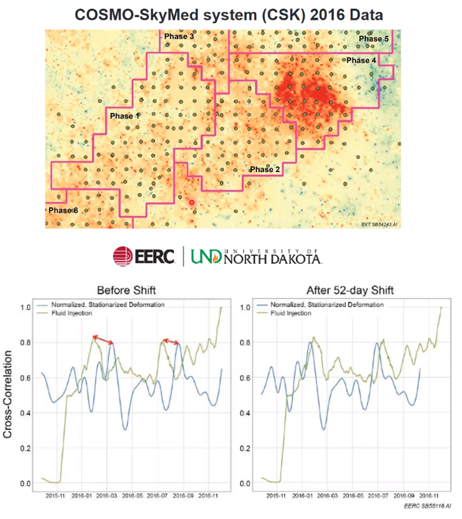
Bell Creek project InSAR data. Surface deformation map (top) showing pronounced deformation associated with phase 4. Correlation of surface deformation and injected volumes (bottom). EERC, PCOR.

There you have it, a quick look at various options for surface and near surface CO2 monitoring as part of an overall MVA program. As I have said before, it seems to me the future is fiber! Next time I will conclude this review of CCUS MVA programs by looking at subsurface evaluation methods. So, yes, more fiber, VSPs, and crosswell tomography.

References

Li et al (2014). A novel shallow well monitoring system for CCUS: with application to Shengli oilfield CO2-EOR project. Energy Procedia. 63. 3956 – 3962. 10.1016/j.egypro.2014.11.425.

Frédérick Gal et al (2019) Soil-Gas Concentrations and Flux Monitoring at the Lacq-Rousse CO2-Geological Storage Pilot Site (French Pyrenean Foreland): From Pre-Injection to Post-Injection. Applied Sciences, MDPI, 2019

Gal, Frederick et al (2014). Study of the environmental variability of gaseous emanations over a CO2 injection pilot—Application to the French Pyrenean foreland. International Journal of Greenhouse Gas Control. 21. 177–190. 10.1016/j.ijggc.2013.12.015.

Pokryszka, Z., Tauziède, C., 2000. Evaluation of gas emission from closed minessurface to atmosphere. In: Environmental Issues and Management Waste inEnergy and Mineral Production, Balkema, Rotterdam, ISBN 9789058090850, pp.327–329. 

Ahmed F., et al. Monitoring of Carbon Dioxide Using Hollow-Core Photonic Crystal Fiber Mach-Zehnder Interferometer. Sensors (Basel). 2019 Jul 31;19(15):3357. doi: 10.3390/s19153357. PMID: 31370157; PMCID: PMC6695808.

Kim, Youjin & He, Wenmei & Yoo, Gayoung. (2019). Suggestions for plant parameters to monitor potential CO 2 leakage from carbon capture and storage (CCS) sites: Original Research Article: Suggested plant parameters to monitor CO 2 leakage from CCS site. Greenhouse Gases: Science and Technology. 9. 10.1002/ghg.1857.

Rucci, S. Cespa and A. Ferretti Reservoir Monitoring using InSAR data: Latest Advances and Future Trends Conference Proceedings, EAGE Workshop on 4D Seismic and Reservoir Monitoring: Bridge from Known to Unknown, Nov 2018, Volume 2018, p.1 – 4

Freifeld BM et al. U-tube: A novel system for acquiring borehole fluid samples from a deep geologic CO2 sequestration experiment. Journal of Geophysical Research 2005